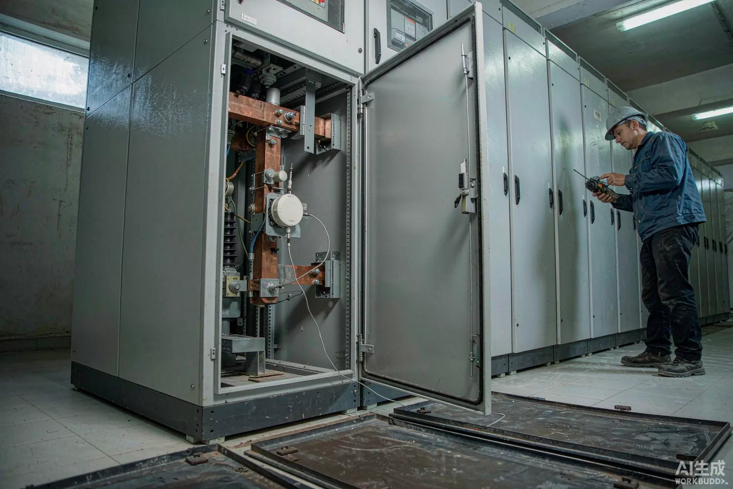
Open the door of a 10 kV switchgear cabinet and the air is busy: corona from busbar edges, switching transients from contactors, AM broadcast leaking in through the cable glands, and the occasional mobile phone. Somewhere in that noise floor is the signal you actually care about — a partial discharge of a few picocoulombs inside a cable termination, a nanosecond-wide burst of energy that widens across the UHF band and repeats twice per power cycle. Catching it early is the difference between a scheduled joint replacement and a busbar fault at three in the morning. This article works through the receive chain of a UHF partial-discharge sensor: what the pulse physically looks like, which front-end parameters decide whether you see it at all, what the newest self-powered and edge-classifying sensors demand from the electronics, and how far domestic parts can carry the design. For the protection stage that normally sits in front of such a receiver, see our limiter diode guide.

Application logic: you are measuring pulses, not a carrier
- The physical event — a partial discharge is an incomplete breakdown in a void or along a surface. It lasts a few nanoseconds and behaves electrically like a current step injected into the winding or the busbar, so its spectrum is broad and extends from a few hundred megahertz to beyond a gigahertz.
- Why the UHF window — below roughly 100 MHz the site is full of corona, thyristor firing and broadcast carriers; the 300 MHz to 1.5 GHz window is comparatively quiet, and the metal enclosure of a GIS or a metal-clad cabinet acts as a natural shield that keeps external interference out. The price of that quiet window is a much smaller signal.
- The sensor — in gas-insulated switchgear the coupler is a disc or a ring electrode mounted inside the tank; in air-insulated cabinets it is a small antenna placed in the gap between the busbar and the earthed shell. Either way the coupling is capacitive and the delivered signal is tiny and extremely short.
- The front end — a limiter to survive the close-in discharge that would otherwise destroy the amplifier, a low-noise stage to lift the pulse above the receiver noise, a band filter to reject out-of-band cellular and broadcast energy, and then either an envelope detector or a direct sampler.
- The detection decision — a detector plus a comparator gives a counted pulse per threshold; a direct sampler gives the pulse shape and therefore the ability to separate a discharge from a switching transient that has a completely different envelope.
- The phase reference — a phase-resolved pattern needs the power-frequency phase. That comes from a voltage divider, a current transformer or an optical sync channel, and the timing accuracy of that reference sets how sharp the resulting pattern is.
- The decision layer — the sensor does not declare a fault. It reports counts, peak levels and a phase histogram, and a monitoring platform applies trend rules and defect classification over weeks.
- The communications layer — most installations run RS-485 to a local unit and then cellular or fibre to the control room; battery sensors use sub-GHz or LoRa links, which pushes the whole power budget back into the front-end design.
The parameters that decide whether you detect or miss a discharge
- Surviving the near-field case — the same sensor must work at 10 metres from a healthy joint and at 10 centimetres from a failing one. A limiter with fast recovery, or a PIN-diode switch that bypasses the amplifier during a strong burst, is not optional.
- Video bandwidth of the detector — an envelope detector with a 1 MHz video bandwidth stretches a 20 ns pulse into something that looks like a 1 microsecond event. That destroys both timing and the ability to count individual discharges in a burst.
- Dynamic range — from the noise floor at minus 90 dBm to a strong internal source at minus 20 dBm is 70 dB. Either a log detector with a wide input range, or a step attenuator switched by a peak detector, is needed to keep the chain linear.
- Noise figure — every decibel of front-end noise is a decibel of lost range. For a passive antenna inside a cabinet the difference between a 1.2 dB and a 3 dB amplifier is roughly 40 percent more usable distance.
- Filter shape — a narrow filter improves rejection but rings, and ringing creates false counts. Choose the bandwidth from the pulse width you must preserve, then add out-of-band rejection in a second stage rather than narrowing the first.
- Timing for localisation — if several sensors are to locate the source by time difference, the timestamp resolution has to be better than a microsecond, which means a common clock and a deterministic trigger path rather than a firmware timestamp.
- Environmental endurance — a cabinet in summer reaches 70 degrees Celsius, an outdoor unit sees minus 40 in the north. Gain drift and detector offset drift with temperature will move every threshold unless they are compensated.
- Long-term stability — a sensor that must run for fifteen years cannot have an electrolytic capacitor in the signal path, and its reference level must not drift enough to trigger an alarm that a maintenance crew will then ignore.
What is changing: arrays, edge classification and self-powered sensors
Three shifts are visible in current utility projects. The first is localisation by array: instead of one sensor per compartment, several couplers share a common clock and the monitoring unit solves for the source position by time difference of arrival. That turns a vague alarm into a pointer at one bay, and it converts the front end into a timing device as much as a measuring device. The second is edge classification: a microcontroller with a modest DSP pipeline now runs feature extraction and a small classifier on the sensor itself, so the uplink carries a label and a confidence rather than a raw waveform. That is a large system-level win because it cuts backhaul traffic and lets a battery sensor sleep between acquisitions. The third is energy autonomy: current-transformer harvesting and, in some designs, RF harvesting remove the aux supply that used to be the reason sensors were only installed where a cabinet had spare terminals.
A fourth change is quieter but consequential: monitoring systems are being folded into substation automation rather than bought as a separate silo. That means the sensor has to speak a standard protocol, present a self-description, and behave predictably on a shared bus — requirements that have nothing to do with RF performance and everything to do with whether the product survives procurement.
Domestic alternatives: suppliers and indicative cost
Be precise about where the domestic supply sits. At system and module level, Chinese suppliers of power-asset monitoring instruments are mature and export widely; a complete UHF sensor is available domestically at competitive prices. At chip level the picture is uneven: general-purpose amplifiers, comparators, references and microcontrollers have domestic families that work well, while wide-dynamic-range logarithmic detectors and low-loss broadband limiters are still dominated by imported parts, and any claim to the contrary should be treated as unverified until you test it yourself.
A realistic domestic front-end: an imported reference low-noise stage such as the PHA-13LN+ for the baseline build, replaced on cost-reduced variants by a SGA5589Z class gain block where noise figure allows; a LFCG-490+ for out-of-band rejection; a COS3502SR as the fast threshold slicer behind the detector; a COS8551TRC zero-drift amplifier for the peak-hold and bias network; an Artery AT32F425C8T7 to sample, timestamp and run the classifier; a HX2001 low-quiescent regulator for the always-on rail; and a TS2502PN array on the antenna port and the RS-485 lines. The pulse-slicing behaviour of the comparator stage is covered in our comparator article.
Price figures below are indicative public-market reference ranges for moderate volumes, compiled from publicly observable listings. They fluctuate with the spot market, package option, grade (industrial, automotive, screened) and order quantity, and must not be read as a quotation. Ask us for a firm price on your exact part numbers and quantities.
| Function (imported anchor) | Example import part / class | Indicative import price (USD) | Domestic candidate | Indicative domestic price (USD) |
|---|---|---|---|---|
| UHF low-noise amplifier | ADI HMC753 class | 6.0 – 12.0 | CETC-institute pHEMT LNA families (family level) | 2.0 – 5.0 |
| Gain block for the second stage | Qorvo SGA5589Z class | 1.2 – 2.5 | Domestic gain block families (family level) | 0.35 – 0.90 |
| Wide-range logarithmic detector | ADI AD8318 class | 8.0 – 16.0 | No volume domestic equivalent identified | — |
| Broadband limiter / protection switch | Imported PIN limiter class | 3.0 – 7.0 | APD0510 class PIN die for a discrete limiter | 0.40 – 1.20 |
| LTCC low-pass filter | Mini-Circuits LFCG class | 1.5 – 3.5 | LFCG-490+ (in stock, imported) | 1.5 – 3.5 |
| Fast comparator | TI TLV3502 class | 0.60 – 1.40 | COS3502SR (Cosine) | 0.12 – 0.30 |
| Zero-drift signal amplifier | ADI AD8551 class | 0.90 – 2.20 | COS8551TRC (Cosine) | 0.15 – 0.40 |
| Control and DSP microcontroller | STM32F4-class Cortex-M4 | 2.0 – 4.5 | AT32F425C8T7 (Artery) | 0.50 – 1.30 |
| Ultra-low quiescent LDO | Imported 1 uA-class LDO | 0.15 – 0.40 | HX2001 (Hexin) | 0.03 – 0.12 |
Where the cost difference actually comes from
The electronics in a UHF partial-discharge sensor are a small fraction of what the utility pays. The money sits in the qualification: cross-comparison with the conventional method, immunity testing in a live substation, a fifteen-year life expectation, and a tender process that asks for three installed references. A domestic bill of materials that is 40 percent cheaper on the board therefore moves the product price by single digits. What the domestic bill of materials buys you is margin headroom for the tender and supply continuity when an imported amplifier goes on allocation, which matters more than the unit saving because these products are bought in projects, not in reels.
The pragmatic split is the one experienced design teams already use: keep the imported logarithmic detector and the first low-noise stage if the specification demands the last two decibels of range, and move every support function — comparators, references, regulators, protection, the microcontroller — to domestic parts where the electrical requirement is easy to meet and the price difference is large in percentage terms. Then qualify a fully domestic variant in parallel for tenders that score local content.
Validation flow before you commit
Inject a known pulse: a calibrated discharge calibrator into a test coupler gives you a repeatable amplitude and a repeatable rise time, which is the only way to separate a front-end problem from a sensor-placement problem. Sweep the input from the noise floor to saturation and plot the transfer curve at three temperatures; a detector that compresses early will under-report strong discharges exactly when they matter. Then run a burst test — fifty pulses in a millisecond — and check that the counter counts fifty rather than one. Finally, install two units side by side, one imported reference and one domestic build, and let them log for a month in the same cabinet; the trend lines, not the spot readings, are what the monitoring platform will act on.
Frequently asked questions
Can a UHF sensor report a discharge level in picocoulombs?
Not absolutely. The UHF method measures radiated energy, so its output is a relative level in dBm plus a count rate; the conversion to picocoulombs depends on the coupler and the enclosure and is normally established by comparison with the conventional method on the same object.
How many sensors does one switchgear room need?
Enough that every compartment is within coupling range of at least one coupler; three per bay is a common starting point for localisation, because two sensors give a hyperbola and three give a unique point.
Why not simply use an oscilloscope-grade sampler everywhere?
Because a sampler that preserves a nanosecond pulse needs a fast converter, a fast clock and a lot of power. Most battery and CT-powered sensors use an envelope detector for the alarm decision and reserve sampling for a triggered capture window.
Do domestic amplifiers have enough bandwidth for the UHF window?
Bandwidth is rarely the limit; noise figure, gain flatness and survives-a-strong-pulse behaviour are. Ask for measured data on your own board over temperature rather than relying on a headline bandwidth.
About us & trademarks: JTDZ Tech (Shenzhen Jingteng Electronics Technology Co., Ltd.) is an independent distributor of electronic components. We are not an authorised distributor or representative of the imported manufacturers named in this article. Manufacturer, brand and part names are used for identification purposes only; all trademarks remain the property of their respective owners. Cross-reference information in this article is based on publicly available sources, is subject to change, and is not a substitute for your own engineering validation. Always verify specifications against the manufacturer's datasheet before design-in or purchase.